To submit questions for the FAQ, simply e-mail Send Questions to GSOLVER@gsolver.com with FAQ in the subject line.
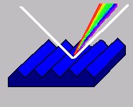
GSOLVER calculates diffraction efficiencies for a general (arbitrary profile and/or construction) periodic diffraction grating illuminated by a monochromatic, plane wave.
Diffraction efficiency is defined in the usual way. Assume that the incident plane wave vector k1 has vector components [k1x, k1y, k1z], and the complex (electric field) amplitude of the (i, j)th diffracted wave is Rij, then the diffraction efficiency (DE) is defined as
DEij=|Rij|2 Re(kzij/k1z)where Re(.) is the real part, and ij is the index of the ijth order (two indexes are needed for crossed gratings). For the transmitted orders k1z is replaced by k3z, the z component of the magnitude of the transmitted 0 order field. [Back to the top]
GSOLVER allows arbitrary polarization defined by the angles (alpha, beta) (including elliptical). See the article at Polarization
[Back to the top]Gratings exist at the planar interface between two infinite half spaces, the superstrate, and the substrate. The superstrate is characterized by a single real number, it's index of refraction. The superstrate must be non absorbing. The substrate is characterized by a real or complex index of refraction. If the substrate is absorptive, then the transmitted diffraction orders are defined at the top surface of the substrate, where they decay exponentially away as they propagate down into the substrate.
The grating region consists of an arbitrary number of material layers that sit on top of the substrate. The superstrate sits on top of the grating layers. Each (arbitrary thickness) layer of the grating consists of a number of uniform materials that are repeated periodic with a period P (the same for all layers). For a traditional grating the layer is periodic in X and uniform in Y. For crossed gratings the layer is periodic in X and (independently) in Y. Each material is characterized by a real or complex index of refraction.
In the GSOLVER EDITOR, the layer view (on the left) is a representation of a single period of a layer. A uniform layer has no index (of refraction) transitions, and is a thin film layer. A binary layer has one index transition (per period). A binary grating can be constructed from such a single layer.
By stacking up layers, and adjusting layer properties, any grating profile can be approximated. By making the uniform regions small enough, any degree of approximation can be achieved. For example, a classical blazed profile might consist of 20 layers. GSOLVER has a number of predefined EDITOR tools to generate common profiles.
[Back to the top]When you generate a new layer, the uniform material regions take default values (using the superstrate and substrate refractive indices). To change these values, scroll to the desired layer and click on the region. The current index of refraction will be placed in the text edit boxes below the layer view. Simply enter new N and K values (use the 'enter' key to update values).
Thus a binary grating with an overlay consists of two layers, a binary layer and a uniform layer. Put the binary layer down first, change the region that has been 'filled in' with the overlay material to the appropriate index of refraction (the same as the overlay material). Then apply a uniform layer and adjust it's index of refraction and thickness as desired.
[Back to the top]On the RUN tab there are two thickness variation parameters, Total Depth, and Link Depth. Selecting Total Depth, the thickness of the full grating (layer stack) is varied, while retained the relative thickness of each layer. Selecting Link Depth, the total thickness of the 'Depth Link List' is varied (while maintaining relative thicknesses of the linked layers). The layers that are not on the depth link list remain unchanged during the DE calculation
To enter a layer in the depth link list click on the Links menu item (while in the EDITOR tab view). This will bring up the links dialog. There are two options, DC and Depth. Click on the Depths option. A list of all the grating layers appears. Select the layers your want to vary. Selected layers are marked with a '+'.
[Back to the top]A duty cycle (DC) is the relative position of an index of refraction transition defined by it's two boundaries. Thus for a binary grating the DC is the relative position of the one index transition bounded by 0 on the left and 1 on the right (positions within the grating are relative to one Period, so the value on the right is always 1). A value of 0.5 means that the binary transition occurs at 50% of the period. For a layer that has multiple index of refraction transitions, say at 0.25, 0.5, and 0.75, the 0.25 transition is bounded by 0 and 0.5. Varying this index transition point from 0 to 100% will move it from 0 to 0.5 (uniformly).
[Back to the top]To select a DC to vary, click on the
Links
menu item from within the EDITOR view. This will bring up the Links dialog. Click on the DC button. A list of all the variable index transitions, for every layer is listed, together with the boundary transition points. Selecting a particular DC is indicated with a + sign. On the RUN view the DC parameter allows one to calculate the DE as the selected DCs are varied from 0 to 100% of their boundary transition points. [Back to the top]The DRUDE model is a simple two parameter model (see the Help file) of the index of refraction. The parameters in GSOLVER were compiled from the literature for fits made to measurements of the various materials (mostly metals) in the infrared. One should expect that these values should be only approximately true, below the first resonance of the material. For accurate values of the index of refraction one should use a Table model where the values of the wavelength together with n and k are entered in a file. GSOLVER linearly interpolates between values as need.
[Back to the top]Since GSOLVER linearly interpolates between entered values of the index of refraction, it is not possible to determine off table values. Usually GSOLVER will return the endpoint value and proceed. It is up to the user to make sure that the table values needed are available for the given calculation.
Table wavelength values have units of microns, and may be entered with a text editor (of the GSOLVER.INI file), or with the GSOLVER materials editor (on the EDITOR tab).
[Back to the top]The Table model is a simple list of wavlengths (in microns), n, k, where the wavelengths are entered in strictly descending order (short to long). GSOLVER looks for a required wavelength by searching the table from top to bottom, finding the entries that bound the given wavelength. A linear interpolation is then made on the n and k values.
[Back to the top]GSOLVER solves the full vector Maxwell's equations for each grating layer. The fields are then matched across each boundary giving the fields in the superstrate and substrate. The diffraction efficiency is then determined for each real propagating order.
The first order Maxwell's equations are written down using a fourier decomposition of the permitivity (and impermitivity) in each layer. The curl equations are used to eliminate the H field giving equations in the E fields. The fourier expansion leads to a set of coupled first order equations. There are 2N+1 equations for each vector component of the E field, where N is the number of orders retained. For TE polarization there is one non-zero vector component. For TM polarization there are two, and for arbitrary polarization there are three. GSOLVER takes the number of non-zero component into account. Thus TE mode is solved much faster than the other polarization cases.
The set of coupled equations are solved via standard algebraic eigen matrix methods. These algorithms require order M3 (order M6) for crossed gratings!) operations, where M is the number of eigenvectors. Double precision arithmetic is used. See the article at Precision
The TE polarization generally converges faster than the TM or arbitrary polarization because there is only one E field component to solve for. Other factors also enter in determining the rate of convergence of the series. It has been seen that the resulting DE series varies in convergence properties from as fast as exponential like, to as slow as 1/n like.
The relative E fields are solved for in each layer. The boundary conditions are then applied iteratively to solve for the magnitude of the fields in the superstrate and substrate (at the interface boundary). The algorithm used to solve for the boundary condition requires taking the inverse of some matrix (of the same order as the eigenmatrix problem), another order M3 problem, one for each interface. Stack matrix methods are used to solve this part of the problem which have been found to be much more stable than Gaussian elimination with pivoting.
Convergence is enhanced by forcing the impermitivity matrix to be and exact inverse of the permitivity regardless of truncation order. For TE and TM this requires taking the inverse of a Toeplitz matrix, an order M2 problem.
[Back to the top]For moderate sized problems several large eigenmatrix problems are solved together with several large matrix inverses. Although the algorithms used are 'industry standard' and highly optimized, roundoff, and multiply-accumulate errors get propagated through to the solution. A DE>1 is nonphysical and indicates that something has gone wrong (energy is conserved by this algorithm implementation so the SUM of the DEs should = 1).
The easiest way to estimate the rate of convergence, and to get a handle on the numerical accuracy of the solution is to pick a representative point in the grating parameter space, and calculation the DE as a function of ORDERS only. A plot of DE vs. ORDERS retained will give an illustration of the convergence properties of the solution. Sometimes, when a DE>1 is encounter a very small change in the parameters, and/or increasing or decreasing the number of orders is sufficient to get the algorithm to behave itself.
The rate of convergence is physically tied to the strength of the evanescent fields supported by the grating. It has been seen that for large evanescent fields the convergence may be as slow as 1/n. This can occur for gratings with large phase shifts (such as metals), and multiple vector components (TM or arbitrary polarization). Examples include metal gratings in TM polarization working in high order. Other algorithms are better suited for such gratings of certain classical profile (piecewise linear, such as a blaze grating). These methods include the 'Integral methods,' and 'exact eigenfunction' methods.
For dielectric gratings, usually only a few evanescent orders are needed (a few more orders more than the number of real propagating orders) since the evanescent field magnitudes decay rapidly in higher order. In these cases only a few more orders need to be retained than the last order that carries any significant field amplitude whether it is real or imaginary.
[Back to the top]Crossed gratings require (2N+1)2 equations (where N is the number of orders retained) for each nonzero vector field component. The rate of growth of the size of the eigenmatrix problem is significant. The amount of memory required by GSOLVER is estimated on the RUN tab. When a large problem is defined, it simply takes a great deal of computer time to calculate. For crossed gratings the time grows quadratically (order of N6) with the number of orders retained. In crossed grating cases it is recommended that GSOLVER be used for problems that require only a few orders.
[Back to the top]GSOLVER does not check the amount of physical RAM available on the machine, other than to report it's size. If the grating problem requires more RAM than is physically available, then Windows (R) will create a swap file, and there will be a great deal of disk access during the solution phase. This will significantly slow the solution progress. It is highly recommended that this situation be avoided, and that the user provide enough physical RAM. Generally grating problems that can be solved without running into numerical problems are smaller than 100Mb.
[Back to the top]Prior versions of GSOLVER used an ASCII grating definition format. This format is convenient for generating grating definitions outside of GSOLVER with some other program (automatic user defined profile generation). This feature is retained in current versions of GSOLVER through the Convert menu item.
There is an article on converting the grating definition in the Help. Each grating definition comes with 13 parameters, and a nested list of layer properties (thickness, followed by index transition points, and index of refraction values). Following is a description of the ASCII grating file format. By exporting simple gratings from GSOLVER, one can examine the resulting ASCII file to clarify this construction.
The *.GSE file format contains a grating description in text format (ASCII). Files may be created outside of GSOLVER with another program (like Mathcad, Matlab, Mathematica, Maple, or any other), and then read into GSOLVER for analysis.
The GSE file format is a list of numbers. These numbers may
be delimited with spaces, tabs, CR/LF, or comma�s; white space
is ignored, and may be used to make the file more readable if
desired. Below is a detailed description of the GSE file entries.
comment line 1 [the first seven lines are reserved for]
comment line 2 [user comments, they are skipped over]
comment line 3 [on file read so anything may be place]
comment line 4 [here]
comment line 5
comment line 6
comment line 7
Theta [degrees]
Phi [degrees]
Alpha [degrees]
Beta [degrees]
Gdim [a 1(thinfilms), 2(normal), or 3(crossed)]
Numlevels [number of layers]
Orders [initial number of orders]
SubstrateN [index (n) of the substrate]
SuperstrateN [index (n) of the superstrate]
SubstrateK [index (k) of substrate]
lambda [wavelength (micrometers)]
LambdaX [X-period (micrometers)]
LambdaY [Y-period (micrometers)=1for Gdim=1,2]
size-5 [Number of remaining entries minus 5]
[the remaining entries are grouped by layer, starting at the substrate and
moving up]
[X,Y are normalized to the (X,Y)Period]
[then comes a nested loop for each region
specifying the Index of refraction (n>0,k>=0)]
Since there are a very large number of ways of presenting multi-dimensional data, no attempt is made in GSOLVER to provide for other than two dimensional plots. In order to make multi-dimensional plots, or otherwise extend data manipulation simply export the grating grid data to your desired data processing tool (such as Excel, or Matlab, etc.).
[Back to the top]GSOLVER solves Maxwell's equations within each grating layer, and applies the boundary conditions between grating layers. These procedures are rigorous up to some truncation order. The numerical accuracy of these procedures is limited by the finite floating point data word, and the truncation order (number of orders retained). Some care given in ascertaining convergence character by examining DE as a function of orders retained will suggest what degree of confidence to give to the numerical results.
[Back to the top]It is interesting that in some cases there can be significant sensitivity to DE based on small deviations in grating structure. It is usually important that the physical grating to be modeled be carefully measured so that it can be accurately modeled in GSOLVER. Often, a study needs to be conducted to ascertain the level of approximation needed to determine the sensitivity of DE to feature size.
For example, simply assuming that a grating is sinusoidal, because it was manufactured by exposing a photoresist to a laser interference pattern, and etching is highly suspect. Such a manufacturing process is highly nonlinear. Several studies have shown that the resulting grating usually contains higher order spatial harmonics that contribute significantly to the DE.
[Back to the top]A diffraction efficiency, DE > 1, means that the point solution was dominated by roundoff and/or numerical truncation error. For large matrix problems finite arithmetic may lead to substantial calculational errors. The first thing to try when this happens is to alter the wavelength, and/or period, and/or number of orders (1 more or less) and see if that helps. Often it is sufficient to simply alter the wavelength by a small amount. Even so, if convergence is very slow (determined by a plot of DE vs. orders retained), the eigenmatrix, or matrix inversion steps may be (or close to being) ill conditioned and limited by the 64 bit floating point data word.
[Back to the top]GSOLVER was originally built for analysis of grating structures with no known analytic eigensolution. Structures in dielectrics (waveguide couplers, subwavelength antireflection gratings, etc.) with complicated material structures were the target problems. This required that the GSOLVER interface and algorithm be driven by the most general point of view.
The classic class of gratings (blazed in metal) is known to have analytic eigensolutions. Spectroscopist working in instrument design constrained by classical approaches are encouraged to apply those methods as one would expect that exact solutions offer more robust calculational approaches.
On the other hand, as modern lithographic and coating techniques expand beyond the semiconductor fabs, new design freedom becomes available to the optical designer. One usually is interested in maximizing (or minimizing) efficiency and dispersion. The past decades have seen the development of dielectric grating structures that exceed the efficiency and other performance measures of blazed gratings in metals, as well as highly specialized grating structures that are readily analyzed by GSOLVER.
[Back to the top]Since GSOLVER incorporates a full vector, rigorous diffraction efficiency solver it seemed natural to include the crossed grating case for completeness. In this case, the number of orders is quadratic in the Orders retained (there are two spatial degrees of freedom). Thus all the memory, and time requirements grow quadratically (very fast) with orders retained. This can be seen by setting up a crossed grating structure and looking at the estimate of the required memory as the orders parameter is increased. 7 orders retained already require more than 100MB of RAM. This suggest that crossed gratings with no more than 1 or 2 real propagating orders might be analyzed, depending on the strength of the evanescent fields supported by the grating interface. Even so, this represents the upper limit. I am aware of some who have used GSOLVER to analyze crossed grating structures that require much more RAM than this, and they have reported that theory and measurement were in good agreement. However, this seems to be pushing the present PC computing architecture to the limit. (Intel now has a 64 bit chip, and there are 64 bit OS's to go with it. So one should expect that as compiler and hardware technology advance, the computational potential of such programs like GSOLVER will continue to improve.)
[Back to the top]The point here is that a uniformly sampled DE curve in wavenumber space is not uniformly sampled in wavelength space. In order to alter the sampling in wavelength space so that a plot looks uniformly sampled in wavenumber space one needs to set up a Parameter Run file. An example of this ships with GSOLVER (test.prm). This file is a simple listing of the 10 GSOLVER parameters, one set for each loop through the DE calculation. Construct a file that has the wavelength sample points desired.
Using this approach, any set of algebraic constraints between the parameters can be constructed. For example a Littrow mount (where wavelength and angle are coupled) is readily applied using the FileRUN feature. (See FileRUN question.)
[Back to the top]The FileRUN button brings up a dialog box that asks the user to select a *.prm file (parameter file). This file is an ASCII file that list the parameters for each DE calculation. There are 10 parameters than may be varied. A single RUN is a calculation of the DE for all orders for the given set of parameters. The file test.prm that ships with GSOLVER is an example of a parameter file, and includes comments on how to modify it.
[Back to the top]Yes. The simplest 'grating' structure is a simple uniform layer (the period is arbitrary, since this structure is periodic on every spatial scale). Thin film stacks may be analyzed, and optimized using the GSOLVER differential evolution algorithm, for example.
[Back to the top]Not yet. This is on our 'to do' list. There are three parts to this problem. This first is to optimize the DE over a range of parameters, and find the best parameter set. This can already be done. Whatever parameter set is selected on the RUN tab will be used to find best fit to the DE goals. For example if both theta and Total Depth are checked (with some range), the results of the Genetic Algorithm RUN (GenRun) will contain the best angle and best total grating depth found. Multiple runs may not result in the same solution since the parameter space is searched in a constrained random manner.
The second part of this problem is to apply an algebraic constraint between the selected parameters, much like in the FileRUN feature. This will be added in the near future. As an aside some have asked that the optimization be on some algebraic combinations of the DE between the orders. This will be incorporated 'later on'. An example of this would be to find a grating where the 1T order is .5*1R order (for example 1T-1R/2=0). Suggestions are welcome on what is desired for this feature.
The third part to this question is to optimize some grating feature over a set of parameters (instead of finding the best parameter set). For example, find the best grating DC in some set of layers that maximizes the DE over a range of wavelengths and angles. As this problem becomes formalized sufficiently to program, it will be added to GSOLVER.
[Back to the top]This depends on the strength of the evanescent fields. This is driven by the magnitude of the phase shifts between the E-fields at the boundary layers. Generally metals support larger evanescent fields. For dielectrics I suggest that one start with a few more orders than the number of real propagating orders (this is the number estimated by GSOLVER, based on the grating equation at the bottom of the RUN tab). Another approach, which is very cumbersome is to look at the actual E-fields using the 'Write Fields to File' feature. A sign of convergence is that the high order fields are much smaller than the low order fields. Alternatively, and easier is to simply plot the DE for each real order as a function of orders retained. This curve should settle down to some constant value. In some cases it seems to oscillate about some constant value, from which an idea of numerical error might be taken. In the worst cases, the algorithm diverges because of round off error. Higher precision arithmetic will be added to GSOLVER as it becomes available from the Compiler and hardware manufacturers (for the PC).
[Back to the top]This happened because the C++ Standards committee defined the long double type to be equivalent to the double (64bits each). The long double use to be 80bits, and is supported by the Intel hardware. However, after the new standard, the compiler manufacturers, for some reason, quickly dropped all support for the 80 bit data type. Hopefully as the processing bandwidth of the PC improves, newer data types will be defined and supported. A 124 bit long double (as in other architectures), or even a 256 long long double would be nice. Such a feature is expected to significantly improve the convergence performance of the algorithms used by GSOVLER.
[Back to the top]See the Polarization article.
[Back to the top]Phase is not defined for the DE, only for the complex fields. The fields may be written to a text file with the 'Write Fields to File' feature. After the RUN, the field values (at the top and bottom interface to the superstrate and substrate) are written. These field values are the coefficients to the plane wave expansion of the diffracted (and evanescent) fields. However, since the eigenvalues are normalized within each layer, the calculated fields are also normalized (by some unknown complex number). It is reasonable to look at the relative phases between diffracted orders (either reflected or transmitted) since this operation is independent of any normalization. GSOLVER does not incorporate any automatic phase calculation.
[Back to the top]A Gaussian beam (or any other type of illumination) may be decomposed (sampled) in wavevector space. That is, a Gaussian consits of a weighted sum of plane waves. It is a simple matter to select the sampling of the incident illumination, and calculate the DE for each wave component, and sum up the results appropriately.
[Back to the top]Only if it (like any other algorithm approach) is poorly implemented. This claim has appeared at various times in the literature, but is unfounded as it describes a particular implementation. The Coupled-Wave algorithm is based on firmly established algebraic techniques for solving a set of coupled differential equations. The problem probably arrises from implementers that fail to calculate normalized eigenvalues (since exponential functions of some eigenvalue times layer depth are formed).
In GSOLVER, it is a simple matter to look at say a binary grating in metal and run the calculation over depth. Using a 1 micron period, Aluminum substrate, the calculation coverges nicely for both TE and TM for depths greater that 106 microns (a meter deep!) though this type of grating behaves the same as an infinite depth grating for depths as 'shallow' as 500 microns.
[Back to the top]The 32 bit key must be installed on the parallel port. Distribution CD's dated prior to August 2001 supplied Rainbow (or Sentinel) driver 8.15. The most up to date driver may be downloaded directly from Rainbow Technology's web page. In the past the driver was supplied with the GSOLVER update file. However, since the driver, together with related support software for the various Windows operating systems is so large, the driver is no longer included with the web download. It is included with the GSOLVER distribution CD.
[Back to the top]