
Grating Solver Development Company
Binary Grating Example:
This section gives a step-by-step example for creating a single binary layer grating (one layer with one index transition).
- Open GsolverV6.1
- The Parameters form is the global settings home. The substrate and superstrate materials may be selected here. (More details are found in the Dialogs chapter of the users manual.) Select a substrate and superstrate material by clicking on the appropriate select buttons.
- Enter the grating period (or lines/mm), wavelength, and other parameters. (A discussion of the angles is given in the Parameters Tab chapter.)
- Click on the Editor tab. Shown on this tab is the graphical working area called the canvas (see chapter 4). The substrate is located at 0 and below, referenced to the ruler on the left, and is not shown on the canvas.
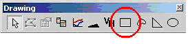
- This example employs the square (rectangle) shape button to draw a rectangular structure. If not already present, use the menu item Tools->Customize to add the drawing tools to the toolbar. (See the section on toolbars if needed.)
-
- Click on the square tool button. Place the mouse cursor anywhere on the active area of the canvas, and, while holding down the left mouse button, drag the mouse to create a rectangle on the canvas.
- Move the mouse cursor into the interior of the rectangle and right click. This brings up an item property menu. Select Properties.
- Select a material for the rectangular region just created. In principle, any shape may be made, and assigned a property. For overlapping shapes, the region on top is used when making the grating definition.
- Drag the rectangle to the bottom of the canvas so it rests on the substrate region.
- The units of the canvas are normalized to 1 grating period. The view region can be sized to any reasonable size, however the width of the canvas is 1 period no matter how the canvas is sized for display purposes. This is explained in detail in the Editor chapter.
- Recalling that periodic boundary conditions are assumed, the single rectangle drawn on the canvas represents a binary grating looking edge on. Once the grating is defined with the graphical editor, an internal piecewise-constant approximation can be created. This gives the representation used in the RCW analysis.
- Click on the Approximation radio button in the upper left corner of the canvas area to create the piecewise constant approximation. Each time this button is clicked, and only then, the internal representation of the piecewise constant construct is recalculated.
- The spatial resolution of the piecewise constant construct is determined by the canvas grid (see Editor Tab for greater detail). It can be made finer in two ways: 1) by changing the grid spacing by selecting Grid Properties from the Grid menu, which can also be activated by right clicking in the canvas area; or 2) by changing the canvas resolution (a number of view units equals one grating period), which can be accessed under the menu entry Edit->Canvas Properties. Also, the actual layer and inter-layer geometric dimensions of any piecewise constant feature are accessible, and modifiable on the Listing/RUN tab.
- Click the Run tab. This brings up the standard global parameter list similar to that of prior versions of GSolver. Using the check boxes, select one or several parameters, enter limits and then click the RUN button. The calculated results are shown on the Results Tab.
- Alternatively, click on the Listing/RUN tab to bring up the single parameter editable list option.
- On the Listing/RUN tab click the Populate button to load the list from the current internal piecewise constant construct. If the ‘Approximation’ button on the Editor form has not been clicked, this construct is empty, and so nothing will change. The piecewise constant listing is discussed in the Listing/RUN chapter.
- For this example the Listing/RUN will be used for a couple of simple calculations. To create a run with the angle of incidence changing. Enter the following formula into grid B2
=D5/2
All cell formulas begin with an equals sign (=) and are calculated immediately. [To toggle between formula view, and value view use the menu Formulas.>Formula View.] The formula engine included in GSolver is very extensive and powerful. It includes all common functions, and logicials, with logical conditional constructs. The formula engine is discussed in the Grid Formula chapter. Any cell can be used in any formula as long as nested iterations and a few restricted cells are avoided. - This Listing/RUN grid comes equipped with a single free parameter in cell D5. Enter the parameter increment and stop values as indicated in E5 and F5; set them to 0 and 80 respectively. This will cause the value of theta (formula entered in B2) to change from 0 to 40 degrees in steps of 0.5 degrees.
- Now click on the RUN button in cell D9. The first thing that happens is that GSolver cycles through the parameter range. For complicated formulas the increment and decrement buttons may be used to single step the grid computation to verify correct behavior.
- After the first run through, the parameter loop is reset, and then on each parameter increment the current grating list, as defined on the grid, is sent to the solver routines. The solution is written to the Results grid (Results tab).
- At the completion of the loop, the Results tab is displayed. Select any column(s) to graph by clicking on their headings. Multiple columns are selected using the shift and ctrl keys along with the mouse in the usual manner. The many options available for graphical display are discussed in the Graphing Options chapter.
- Return to the Listing/RUN tab. Reset the parameter D5 to 0 and change cell B2 to 10 for a fixed 10 degree incidence angle.
- Enter the following formula in cell B6 (wavelength):
=if(D5/100>.5,D5/100,.5)
This is a from of a conditional entry. The wavelength remains constant (0.5 microns) if D5/100<=0.5. Otherwise it changes linearly with D5 as given in the formula. - In cell B7 enter the following formula
=1.+D5/100.
This formula changes the grating period from 1 to 2 linearly as D5 changes from 0 to 100. - Change the orders field to 5.
- Click the Run button and examine the results.